In mathematics, a straight line is represented by the equation $y = mx + c$:
where m is the slope and c is the y-intercept. On paper, this equation allows us to draw a line smoothly, as points on the line can have continuous values (including decimals).
However, in computer graphics, we face a challenge: displays consist of discrete pixels, so lines cannot be drawn with infinite precision. Instead, we must determine which pixels should be colored to best approximate the line. This process is called rasterization.
Bresenham’s line algorithm is a well-known method for rasterizing lines. Let’s derive the key variables and equations for this algorithm using the basic line equation.
Note: A line can fall into one of eight octants, as shown in the image. To derive the equations for the Breshenham line drawing algorithm, we will focus on a line in the first octant, where the slope satisfies 0 ≤ m ≤ 1. Later, we can extend this to derive the equations for other octants.
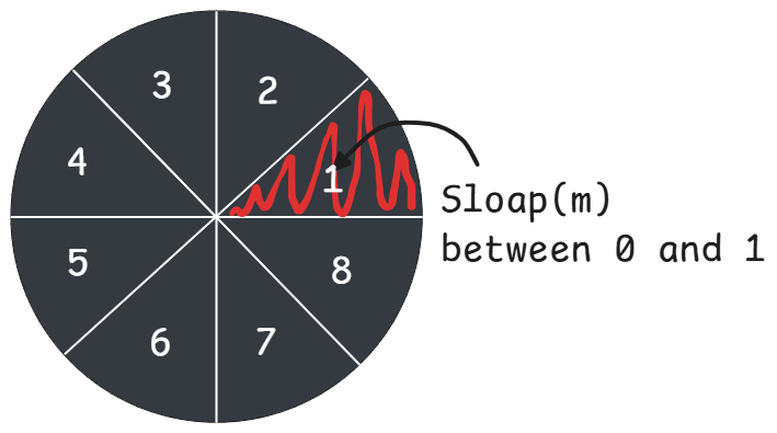
Figure 1
Assumption 1: In computer displays, pixel counting starts from the top-left corner. The x-coordinate increases to the right, and the y-coordinate increases downward. However, for simplicity in deriving equations, let’s assume x and y follow the behavior of standard cartesian coordinates:
Assumption 2: Assume the center of a pixel represents its continuous value. This means the length of the $y_{k}$ pixel is the distance from the bottom-most point of the display to the center of the $y_{k}$ pixel. (See Figure 2)
Understanding Pixel Selection
When drawing a line between two points, the line may pass between pixels. Consider the following situation
As shown in the image below, let’s assume we are currently at the k-th position for both x and y. Our task is to predict the next pixel to draw. Since we are in the first octant, we know the next x-coordinate will be $x_{k}$+1. However, we need to decide whether to color the current $y_{k}$ pixel or the next $y_{k}$ +1 pixel.
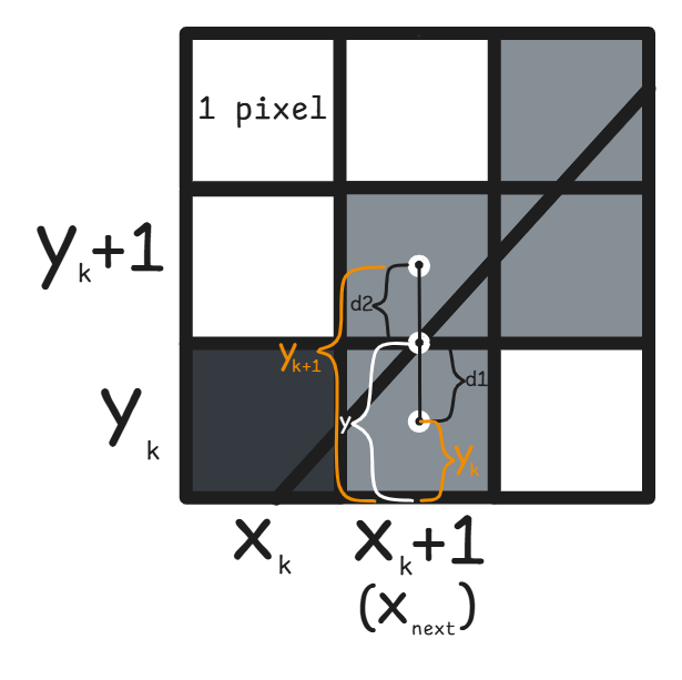
Figure 2
To make this decision, we need to calculate two values, d1 and d2, and choose the pixel that is closer to the actual line to minimize visual error.
We will define this decision as a parameter d, and our goal is to derive d from the line equation $y = mx + c$. Using this parameter, we can determine which y-value to color next.
Derivation of Decision Variable(d)
The line equation is given as $y = mx + c$:
Let the y-coordinate of the current pixel be $y_{k}$, and the next consecutive pixel in the y-direction be $y_{k}$+1($y_{next}$).
Let the x-coordinate of the current pixel be $x_{k}$, and the next consecutive pixel in the x-direction be $x_{k}$+1($x_{next}$).
Define key variables:
$\text{current x} = x_{k}$
$\text{current y} = y_{k}$
$\text{next x} = x_{next} = x_{k} + 1 \text{ always }$
$\text{next y} = y_{next} = y_{k} + 1 \text{ or } y_{k}$
The distances d1 and d2 are defined as:
$y = y_{k} + d_{1}$
$d_{1} = y \text{ } – \text{ } y_{k}$
$y_{k} + 1 = y + d_{2}$
$d_{2} = y_{k} + 1 \text{ } – \text{ } y$
Using the line equation $y = mx + c$
$d_{1} = y \text{ } – \text{ } y_{k }$
$\text{since } y = mx_{\text{next}} + c $
$d_{1} = mx_{\text{next}} + c \text{ } – \text{ } y_{k}$
$d_{2} = y_{k} + 1 \text{ } – \text{ } y$
$\text{since } y = mx_{\text{next}} + c$
$d_{2} = y_{k} + 1 \text{ } – \text{ } (mx_{\text{next}} + c)$
$d_{2} = y_{k} + 1 \text{ } – \text{ } mx_{\text{next}} \text{ } – \text{ } c$
Subtracting d1 from d2:
$d_{1} \text{ } – \text{ } d_{2} = mx_{next} + c \text{ } – \text{ } y_{k} \text{ } – \text{ } (y_{k} + 1 \text{ } – \text{ } mx_{next} \text{ } – \text{ } c) $
$d_{1} \text{ } – \text{ } d_{2} = mx_{next} + c \text{ } – \text{ } y_{k} \text{ } – \text{ } y_{k} \text{ } – \text{ } 1 + mx_{next} + c $
$d_{1} \text{ } – \text{ } d_{2} = 2mx_{next} \text{ } – \text{ } 2y_{k} + 2c \text{ } – \text{ } 1$
Removing the Slope (m)
We need to remove the slope (m) in Bresenham’s Line Algorithm because:
- Avoid Floating-Point Calculations:
The slope \(m = \dfrac{\nabla y}{\nabla x}\) often results in fractional values, requiring floating-point arithmetic. Floating-point operations are slower and less efficient compared to integer arithmetic, especially on older or resource-constrained systems. - Use Only Integers:
By eliminating m, we can reformulate the decision-making process entirely using integers. This makes the algorithm faster and avoids precision errors that can occur with floating-point numbers. - Simplify Computations:
Removing m simplifies the math by focusing only on differences (Δx and Δy) between pixel coordinates. This makes the algorithm easier to implement and more computationally efficient.
\(m = \dfrac{\nabla y}{\nabla x}\)
Substituting m into the equation:
\(\nabla x \times (d_{1} – d_{2}) = (2 \dfrac{\nabla y}{\nabla x} x_{next} – 2y_{k} + 2c – 1) \times \nabla x \)
\(\nabla x \times (d_{1} – d_{2}) = 2 \nabla y x_{next} – 2y_{k} \nabla x + 2c\nabla x – \nabla x \)
\(\nabla x \times (d_{1} – d_{2}) = 2 \nabla y (x_{k} + 1) – 2y_{k} \nabla x + 2c\nabla x – \nabla x \)
\(\nabla x \times (d_{1} – d_{2}) = 2 \nabla y x_{k} + 2 \nabla y – 2y_{k} \nabla x + 2c\nabla x – \nabla x \)
\(\nabla x \times (d_{1} – d_{2}) = 2 \nabla y x_{k} – 2\nabla xy_{k} \textcolor{red}{ + (2 \nabla y + 2c\nabla x – \nabla x)} \)
Ignoring constant terms (as they do not affect the decision-making):
\(\nabla x \times (d_{1} – d_{2}) = 2 \nabla y x_{k} – 2\nabla xy_{k} \)
\(\text{Here we need to know about } (d_{1} – d_{2}) \text{ is } >0 \text{ or } < 0 \)
\(\text{Then we can ignore } \nabla x \)
\(\text{We will take } \nabla x \times (d_{1} – d_{2}) \text{ as } d_{k} (\text{Decision variable k})\)
\(d_{k} = 2 \nabla y x_{k} – 2\nabla xy_{k}\)
\(\text{So } d_{next} = 2 \nabla y x_{next} – 2\nabla xy_{next} \)
Updating the Decision Variable
For the next step, the decision variable \(d_{next}\) is calculated as:
\(d_{next} = 2 \nabla y x_{next} – 2\nabla xy_{next} \)
\(\text{Lets’s subtract } d_{k} \text{ from } d_{next}\)
\(d_{next} – d_{k} = (2 \nabla y x_{next} – 2\nabla xy_{next}) – (2 \nabla y x_{k} – 2\nabla xy_{k}) \)
\(d_{next} – d_{k} = 2 \nabla y x_{next} – 2\nabla xy_{next} – 2 \nabla y x_{k} + 2\nabla xy_{k} \)
\(d_{next} – d_{k} = 2 \nabla y x_{next} – 2 \nabla y x_{k} – 2\nabla xy_{next} + 2\nabla xy_{k} \)
\(d_{next} – d_{k} = 2 \nabla y (x_{next} – x_{k}) – 2\nabla x (y_{next} – y_{k}) \)
\(d_{next} = [2 \nabla y (x_{next} – x_{k}) – 2\nabla x (y_{next} – y_{k})] + d_{k} \)
Depending on the value of \(d_{k}\):
\(\textcolor{black}{\text{If }} \textcolor{red}{d_{k}} < 0 \)
\(y_{next} = y_{k} \)
\(d_{next} = [2 \nabla y (x_{next} – x_{k}) – 2\nabla x (y_{next} – y_{k})] + d_{k} \)
\(d_{next} = [2 \nabla y (x_{k} + 1 – x_{k}) – 2\nabla x (y_{k} – y_{k})] + d_{k} \)
\(d_{next} = 2 \nabla y + d_{k} \)
\(\textcolor{black}{\text{If }} \textcolor{red}{d_{k}} \geq 0 \)
\(y_{next} = y_{k} + 1 \)
\(d_{next} = [2 \nabla y (x_{next} – x_{k}) – 2\nabla x (y_{next} – y_{k})] + d_{k} \)
\(d_{next} = [2 \nabla y (x_{k} + 1 – x_{k}) – 2\nabla x (y_{k} + 1 – y_{k})] + d_{k} \)
\(d_{next} = 2 \nabla y – 2 \nabla x + d_{k} \)
Initializing the Algorithm
To start the algorithm, we calculate the initial decision variable \(d_{1}\):
\(d_{1} = 2 \nabla y x_{1} – 2\nabla xy_{1} \textcolor{red}{ + (2 \nabla y + 2c\nabla x – \nabla x)}\)
\(d_{1} = 2 \nabla y x_{1} – 2\nabla xy_{1} + 2 \nabla y + 2c\nabla x – \nabla x\)
\(\textcolor{black}{\text{Now we have to get rid of }} \textcolor{red}{c} \textcolor{black}{\text{ because it is unknown}} \)
\(d_{1} = 2 \nabla y x_{1} – 2\nabla xy_{1} + 2 \nabla y + 2c\nabla x – \nabla x\)
\(\textcolor{black}{\text{According to }} y = mx+c\)
\(c = y -mx \)
\(m = \dfrac{\nabla y}{\nabla x}\)
\(c=y-\dfrac{\nabla y}{\nabla x}x\)
\(d_{1} = 2 \nabla y x_{1} – 2\nabla xy_{1} + 2 \nabla y + 2c\nabla x – \nabla x \textcolor{black}{\text{ Let’s apply it here,}}\)
\(d_{1} = 2 \nabla y x_{1} – 2\nabla xy_{1} + 2 \nabla y + 2(y_{1}-\dfrac{\nabla y}{\nabla x}x_{1})\nabla x – \nabla x \)
\(d_{1} = 2 \nabla y x_{1} – 2\nabla xy_{1} + 2 \nabla y + 2\nabla x(y_{1}-\dfrac{\nabla y}{\nabla x}x_{1}) – \nabla x \)
\(d_{1} = 2 \nabla y x_{1} – 2\nabla xy_{1} + 2 \nabla y + 2\nabla xy_{1}-\dfrac{\nabla y}{\nabla x}x_{1}2\nabla x – \nabla x \)
\(d_{1} = 2 \nabla y x_{1} – 2\nabla xy_{1} + 2 \nabla y + 2\nabla xy_{1}-
2\nabla yx_{1} – \nabla x \)
\(d_{1} = 2 \nabla y – \nabla x \)
Summary of the Algorithm
- Start at the initial pixel (x0,y0).
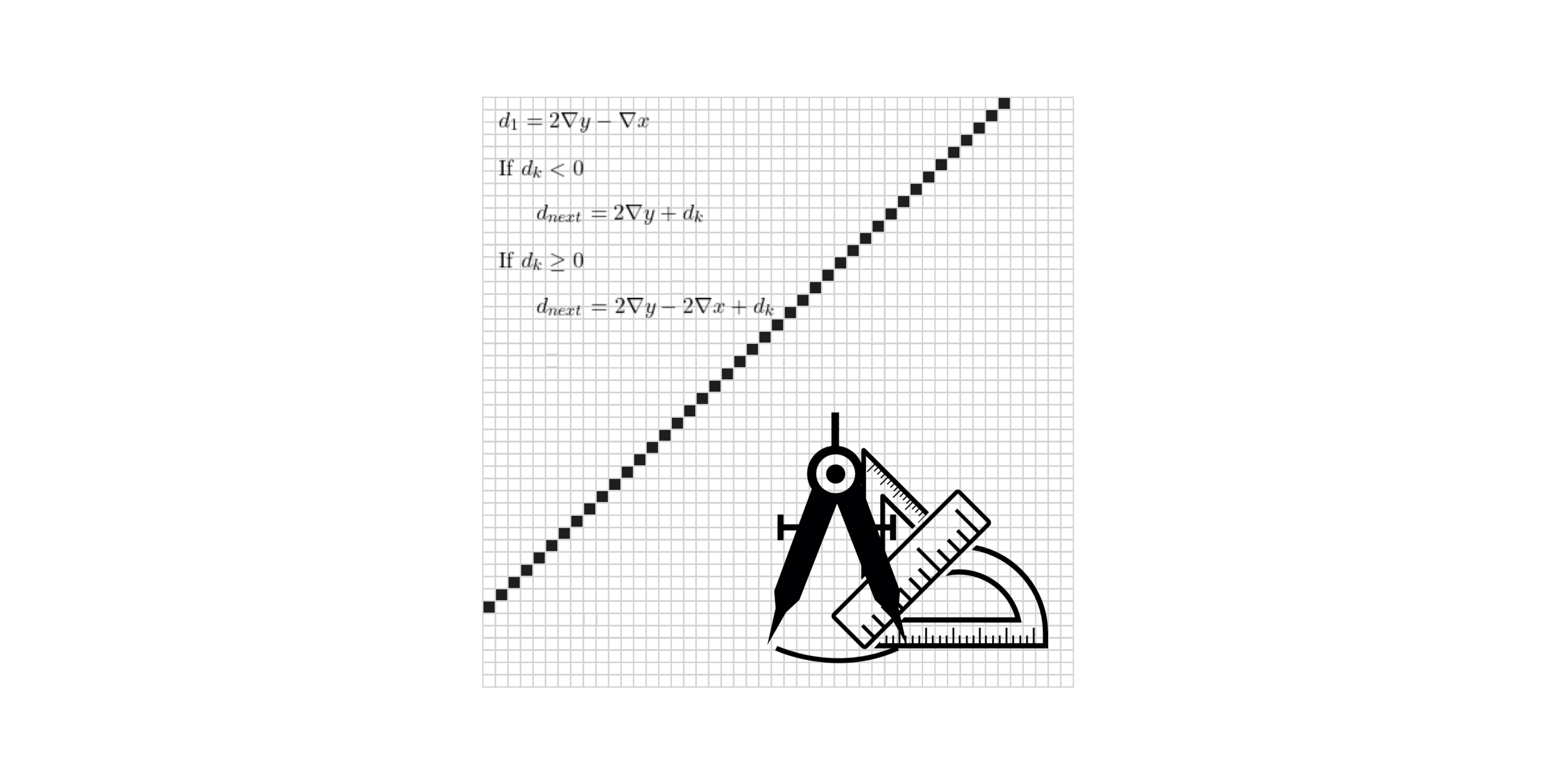
- Compute the initial decision variable: \(d_{1} = 2 \nabla y – \nabla x \)
- At each step, update the decision variable:
- If \(d_{k} < 0\) : Move horizontally, \(d_{next} = 2 \nabla y + d_{k} \).
- If \(d_{k} \geq 0\) : Move diagonally, \(d_{next} = 2 \nabla y – 2 \nabla x + d_{k} \)
4. Repeat until the end of the line.
This method ensures that the line is rasterized efficiently with minimal visual errors.
To derive the decision variable for the 2nd octant, you can follow a similar process as for the 1st octant. In this case:
- The next y-coordinate will always be \(y_{next} = y_{k} + 1\)
- Based on the decision variable, you need to determine whether the next x-coordinate remains the same (\(x_{k}\)) or increments by 1 (\(x_{k} + 1\)).
- If \(d_{k}<0\): Move horizontally, \(d_{next} = d_{k} – 2 \nabla x \).
- If \(d_{k} \geq 0\): Move diagonally, \(d_{next} = 2 \nabla y – 2 \nabla x + d_{k} \)